Methods

To perform its analysis, Susurrant uses a variety of methods derived from digital signal processing (DSP), machine learning, and music information retrieval (MIR). All of these are techniques that can help to derive interesting information from audio.

Most analysis procedures involving machine learning go through several overarching steps:

• feature extraction: turning raw data into a representation more suitable for analysis, typically a numerical vector
• training: “fitting” a model to the data, according to certain parameters
• output: using the trained model to classify examples, make decisions, etc.

Susurrant follows this general pattern; the specifics are outlined below.

• Analysis Pipeline
• Feature Extraction
  • Mel-frequency Cepstral Coefficients
  • Chroma
  • Beat Spectra
• Training: Topic Modeling
  • Caveats
• Results
  • Visualization
  • Sonification
• In Summary

Analysis Pipeline

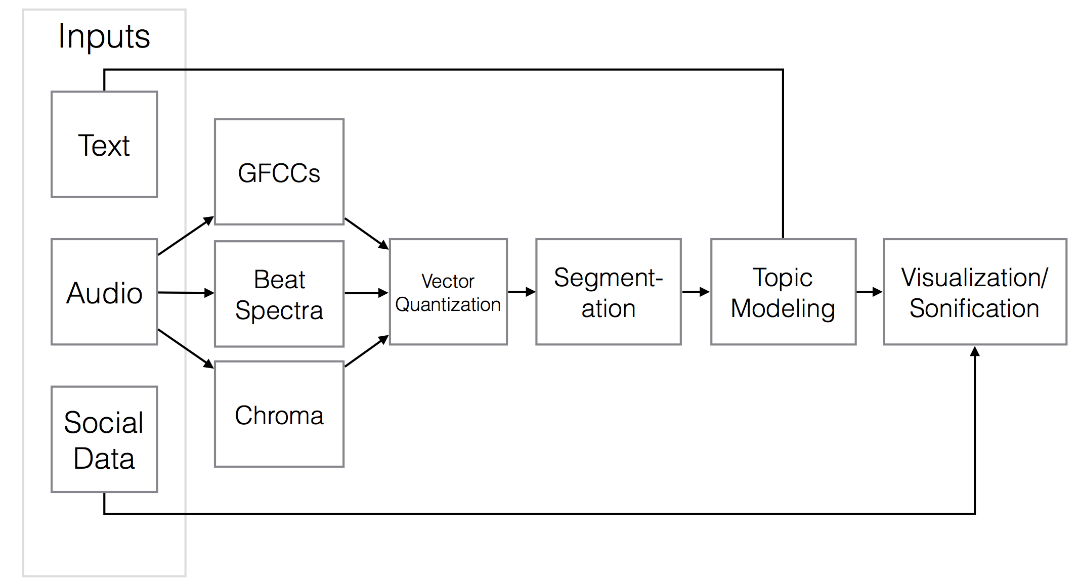
This flowchart illustrates the different stages of Susurrant’s analysis, each of which will be explained in more detail.

Feature Extraction

In the feature extraction phase, Susurrant transforms audio data using the following methods, each of which captures a specific piece of salient information about the audio. At present, Susurrant uses the Essentia library via Python to carry out these analyses.

Mel-frequency Cepstral Coefficients

MFCCs are a measurement of audio’s timbre: is it bright and harsh, or dark and mellow? Often used in speech recognition tasks, the MFCC can distinguish between vowels and consonants; it can also be used to characterize the overall character of sound and (if applicable) its instrumentation.

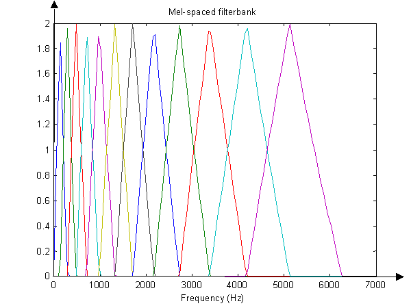
MFCCs can be thought of as a “spectrum of a spectrum.” First, the Fast Fourier transform, used extensively in DSP, transforms an audio signal into the frequency domain. The original time-based signal is analyzed for its intensity across many different frequency bands, in order to produce (for example) the familiar spectrogram. This frequency spectrum is then put through a Mel filterbank: a set of triangular psychoacoustic filters meant to model the frequencies emphasized by the human ear.

Finally, the logarithm of the mel-frequency cepstrum is passed through another transform (the Discrete Cosine Transform). All of these steps have the effect of separating out different components of the original sound’s timbre, in a manner independent of the original sound’s pitch.

The MFCC holds a great deal of information about the intensity and distribution of different frequencies present in the original audio, in a very small space. Often, a vector of only 12 numbers is retained from the 1024 or 2048 samples used in the FFT.

There are, however, limitations to what the MFCC can capture. Compare, for example, the following audio sample with a reconstruction based on its MFCC representation, drawn from Juhan Nam’s Ph.D work:¹

Technically, Susurrant uses “gammatone-frequency cepstral coefficients,”² a very similar feature that uses a slightly different psychoacoustic model. The above limitations still largely apply.

Chroma

Chroma is a measurement of a sound’s intensity at each of the 12 pitch classes associated with Western music. You can imagine that any musical notes and harmonies present in the sound have been mapped onto a single octave of the piano, including both black and white keys.

This feature is less useful outside of musical contexts, but is still often used to characterize the harmonic content of a song.

Beat Spectra

Beat spectra are a way of representing a sound’s similarity to itself over different time scales. They are a form of “autocorrelation,” a method that is typically used to identify the pitch of a sound, but analyzed over several seconds instead of a brief instant. On a larger scale, this process can reveal beats within the metrical structure of music or in non-musical audio that evinces rhythmic repetition.

TODO: visual example of beat spectrum

In Susurrant, the beat spectrum is treated as a signal and then processed through FFT, giving a 24-dimension feature vector (see Foote et al. for more details of this approach).

Training: Topic Modeling

Susurrant uses a technique known as topic modeling to carry out its construction of a concordance of sounds. This procedure models individual “documents” (sounds) as if they were randomly assembled by combining a smaller number of “topics” in different proportions. Each “topic” is made up of a set of “words” (sonic or textual features), each with a different probability of occuring within that topic.

Although this technique is often used for text, as its terminology might suggest, it can also be applied to other forms of data– including audio. Uri Shalit et al. have used an extension of this technique to analyze acoustic evidence of musical influence and change over time within Columbia University’s Million Song Dataset. The simpler technique employed here does not distinguish between audio from different eras or created by different individuals: all sounds are incorporated into a single analysis, which can later be aggregated according to content creators, timespans, or other variables.

Caveats

Note that topic modeling uses a “bag-of-words” model, meaning that it does not pay attention to the order of words or sonic features in its analysis. All that matters for this algorithm is the co-occurrence of certain features somewhere in the same document (for Susurrant, this is an approximately 3-minute segment of audio).

Another important concern: topic modeling is a probabilistic process, meaning that its results will vary (sometimes widely) between different runs of the process. I strongly suggest running through the process several times so that you get a sense of what is “really there,” rather than only a suggestive coincidence.

Results

After a topic model has been trained on the data, Susurrant displays the resulting topics through a browser-based interface. Users can both see graphical representations of the different features associated with each topic, and hear an audio representation of these features.

Visualization

Susurrant uses star plots to generate specific “glyphs” for each sonic feature. Probability is represented through the opacity; fainter shapes are less likely within a topic.

This graphic is not aimed at reading off the numerical values of each feature– indeed, the combined image conflates the axes of radically different feature types, rendering it useless for such a task. Rather, the combined and individual plots allow users to distinguish visually between the different tokens (and to compare tokens within a particular feature type).

For example, here are two chroma features that represent different harmonic content within a sound.

TODO: chroma feature star plots

And here are two GFCC features, showing different distributions of low and high frequencies within a spectrum.

TODO: GFCC feature star plots

Sonification

Perhaps the most novel aspect of Susurrant compared to many other audio analysis tools is its sonification component. Every feature can be hovered over to hear how it sounds in isolation, and the topic overview graphic plays back each of its constituent tokens according to their probability (i.e., if a token has 100% probability, it will be played exclusively; if two tokens are 50%-50%, they will be played equally often; and so on.)

TODO: audio example of sonified topics and tokens

Furthermore, the individual sounds of the corpus can be sonified according to each type of feature. Thus, users can listen to a particular sound in its original form, or as interpreted through its GFCC, chroma, or beat spectral features.

TODO: audio samples of original track, each feature type

In Summary

Each feature type in Susurrant represents a different aspect of sound, which then feeds into its algorithmic analysis. By letting you view and listen to these feature representations, the tool attempts to help you better understand the relationship between your data and the computational analysis that results.